Quick Start with the `difNLR()` function • difNLR

This vignette demonstrates the basic usage of the difNLR() function using example data from the package.

Load package

library(difNLR)

Load data

We here use the GMAT dataset. It is s a generated dataset based on parameters from Graduate Management Admission Test (GMAT, Kingston et al., 1985). First two items were considered to function differently in uniform and non-uniform way respectively. The dataset represents responses of 2,000 subjects to multiple-choice test of 20 items. A correct answer is coded as 1 and incorrect answer as 0. The column group represents group membership, where 0 indicates reference group and 1 indicates focal group. Groups are the same size (i.e. 1,000 per group). The distributions of total scores (sum of correct answers) are the same for both reference and focal group (Martinkova et al., 2017).

data(GMAT)
Data <- GMAT[, 1:20] # binary items
group <- GMAT[, "group"] # group membership variable

summary(Data)

##      Item1           Item2            Item3            Item4      
##  Min.   :0.000   Min.   :0.0000   Min.   :0.0000   Min.   :0.000  
##  1st Qu.:0.000   1st Qu.:0.0000   1st Qu.:0.0000   1st Qu.:1.000  
##  Median :1.000   Median :1.0000   Median :1.0000   Median :1.000  
##  Mean   :0.525   Mean   :0.5695   Mean   :0.7135   Mean   :0.782  
##  3rd Qu.:1.000   3rd Qu.:1.0000   3rd Qu.:1.0000   3rd Qu.:1.000  
##  Max.   :1.000   Max.   :1.0000   Max.   :1.0000   Max.   :1.000  
##      Item5            Item6           Item7            Item8       
##  Min.   :0.0000   Min.   :0.000   Min.   :0.0000   Min.   :0.0000  
##  1st Qu.:1.0000   1st Qu.:0.000   1st Qu.:0.0000   1st Qu.:0.0000  
##  Median :1.0000   Median :1.000   Median :1.0000   Median :1.0000  
##  Mean   :0.8145   Mean   :0.639   Mean   :0.6505   Mean   :0.6175  
##  3rd Qu.:1.0000   3rd Qu.:1.000   3rd Qu.:1.0000   3rd Qu.:1.0000  
##  Max.   :1.0000   Max.   :1.000   Max.   :1.0000   Max.   :1.0000  
##      Item9           Item10           Item11           Item12     
##  Min.   :0.000   Min.   :0.0000   Min.   :0.0000   Min.   :0.000  
##  1st Qu.:0.000   1st Qu.:0.0000   1st Qu.:0.0000   1st Qu.:0.000  
##  Median :1.000   Median :1.0000   Median :1.0000   Median :1.000  
##  Mean   :0.579   Mean   :0.5755   Mean   :0.6745   Mean   :0.548  
##  3rd Qu.:1.000   3rd Qu.:1.0000   3rd Qu.:1.0000   3rd Qu.:1.000  
##  Max.   :1.000   Max.   :1.0000   Max.   :1.0000   Max.   :1.000  
##      Item13          Item14          Item15          Item16      
##  Min.   :0.000   Min.   :0.000   Min.   :0.000   Min.   :0.0000  
##  1st Qu.:0.000   1st Qu.:0.000   1st Qu.:0.000   1st Qu.:0.0000  
##  Median :1.000   Median :0.000   Median :1.000   Median :0.0000  
##  Mean   :0.742   Mean   :0.444   Mean   :0.523   Mean   :0.4475  
##  3rd Qu.:1.000   3rd Qu.:1.000   3rd Qu.:1.000   3rd Qu.:1.0000  
##  Max.   :1.000   Max.   :1.000   Max.   :1.000   Max.   :1.0000  
##      Item17           Item18           Item19           Item20      
##  Min.   :0.0000   Min.   :0.0000   Min.   :0.0000   Min.   :0.0000  
##  1st Qu.:0.0000   1st Qu.:0.0000   1st Qu.:0.0000   1st Qu.:0.0000  
##  Median :0.0000   Median :0.0000   Median :0.0000   Median :0.0000  
##  Mean   :0.4525   Mean   :0.4105   Mean   :0.4825   Mean   :0.4125  
##  3rd Qu.:1.0000   3rd Qu.:1.0000   3rd Qu.:1.0000   3rd Qu.:1.0000  
##  Max.   :1.0000   Max.   :1.0000   Max.   :1.0000   Max.   :1.0000

table(group)

## group
##    0    1 
## 1000 1000

DIF detection with generalized logistic regression models

Not constrained 4 parameter logistic (PL) model using the IRT parametrization is of the following form: $\begin{align} P(Y_{pi} = 1 \mid X_p, G_p) =& (c_{i} + c_{i\text{DIF}} \cdot G_p) + (d_{i} + d_{i\text{DIF}} \cdot G_p - c_{i} - c_{i\text{DIF}} \cdot G_p) / \\ &(1 + \exp(-(a_i + a_{i\text{DIF}} \cdot G_p) \cdot (X_p - b_p - b_{i\text{DIF}} \cdot G_p))), \end{align}$ where $X_p$ is the matching criterion (e.g., standardized total score) and $G_p$ is a group membership variable for respondent $p$ . Parameters $a_i$ , $b_i$ , $c_i$ , and $d_i$ are discrimination, difficulty, guessing, and inattention for the reference group for item $i$ . Terms $a_{i\text{DIF}}$ , $b_{i\text{DIF}}$ , $c_{i\text{DIF}}$ , and $d_{i\text{DIF}}$ then represent differences between the focal and reference groups in discrimination, difficulty, guessing, and inattention for item $i$ , respectively.

To perform DIF detection, besides Data and group variable, we need to specify the name of the focal group with the argument focal.name and the generalized regression model through the model argument. The options are as follows: for 1PL model with discrimination parameter fixed on value 1 for both groups, for 1PL model with discrimination parameter set the same for both groups, for logistic regression model, for 3PL model with fixed guessing for both groups, for 3PL model with fixed inattention for both groups, (alternatively also ) for 3PL regression model with guessing parameter, for 3PL model with inattention parameter, for 4PL model with fixed guessing and inattention parameter for both groups, (alternatively also ) for 4PL model with fixed guessing for both groups, (alternatively also ) for 4PL model with fixed inattention for both groups, or for 4PL model.

Here we use the 3PL model with the same guessing parameter $c_i$ for both groups on the GMAT dataset.

(x <- difNLR(Data, group, focal.name = 1, model = "3PLcg"))

## Detection of all types of differential item functioning
## using the generalized logistic regression model
## 
## Generalized logistic regression likelihood ratio chi-square statistics
## based on 3PL model with fixed guessing for groups 
## 
## Parameters were estimated using non-linear least squares
## 
## Item purification was not applied
## No p-value adjustment for multiple comparisons
## 
##        Chisq-value P-value    
## Item1  82.0689      0.0000 ***
## Item2  28.3232      0.0000 ***
## Item3   0.6845      0.7102    
## Item4   3.3055      0.1915    
## Item5   1.1984      0.5492    
## Item6   0.1573      0.9244    
## Item7   8.3032      0.0157 *  
## Item8   2.8660      0.2386    
## Item9   0.4549      0.7966    
## Item10  1.3507      0.5090    
## Item11  1.2431      0.5371    
## Item12  1.0537      0.5905    
## Item13  4.4139      0.1100    
## Item14  1.4940      0.4738    
## Item15  1.3079      0.5200    
## Item16  0.1424      0.9313    
## Item17  3.1673      0.2052    
## Item18  2.0206      0.3641    
## Item19  6.2546      0.0438 *  
## Item20  3.4871      0.1749    
## 
## Signif. codes: 0 '***' 0.001 '**' 0.01 '*' 0.05 '.' 0.1 ' ' 1
## 
## Detection thresholds: 5.9915 (significance level: 0.05)
## 
## Items detected as DIF items:
##  Item1
##  Item2
##  Item7
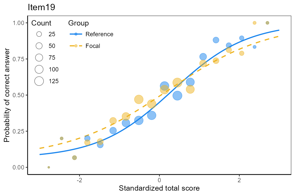
##  Item19

The functions computes $\chi^2$ -statistics and corresponding p-values, suggesting items 1, 2, 7, and 19 to function differently for the reference and focal groups.

Plot item characteristic curves

We plot item characteristic curves for DIF items.

plot(x, item = x$DIFitems)

## $Item1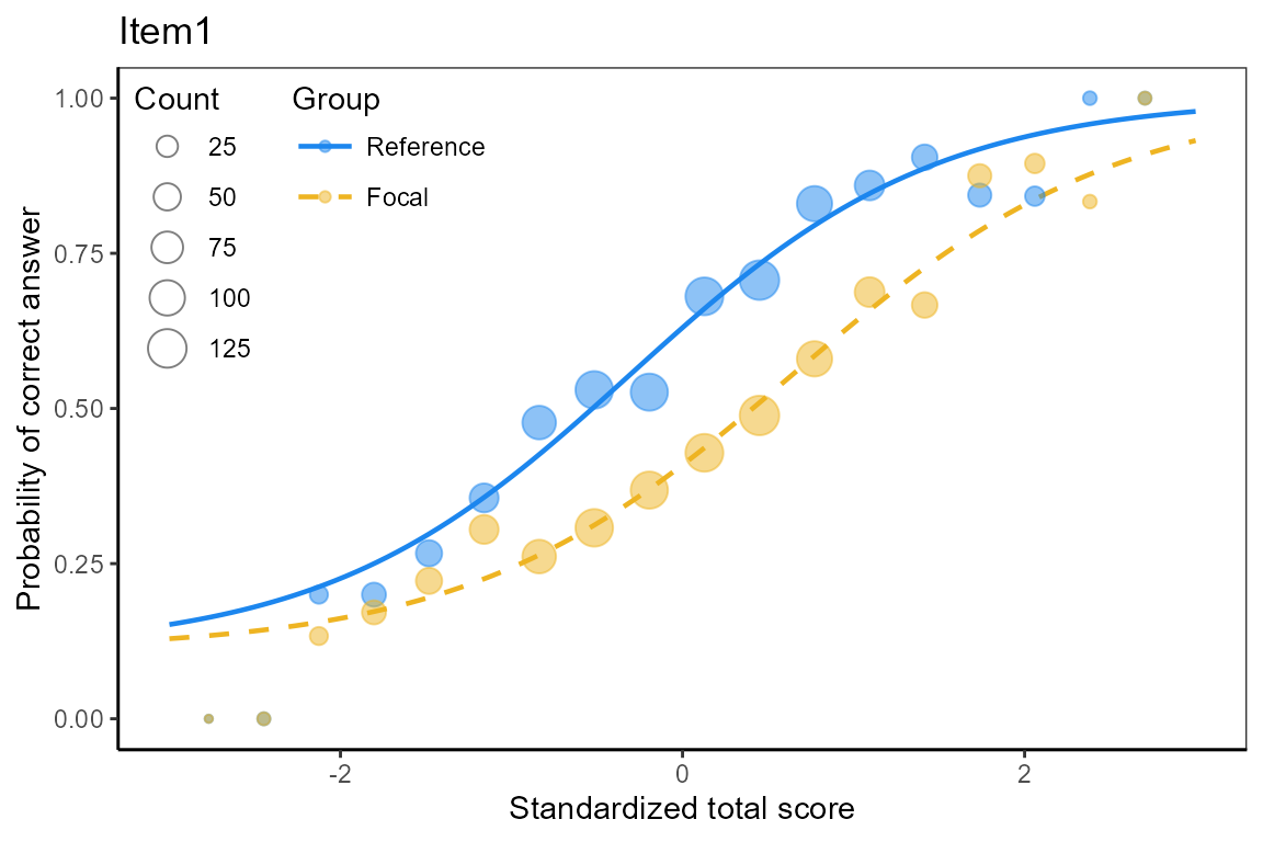

## 
## $Item2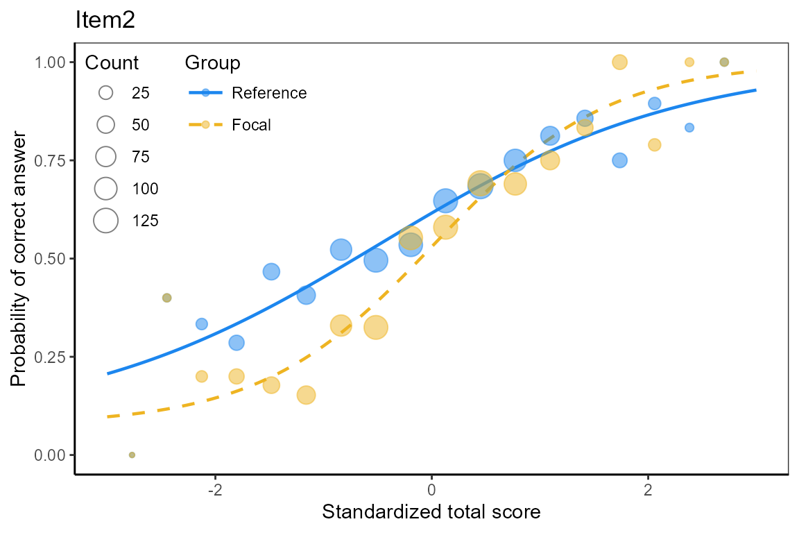

## 
## $Item7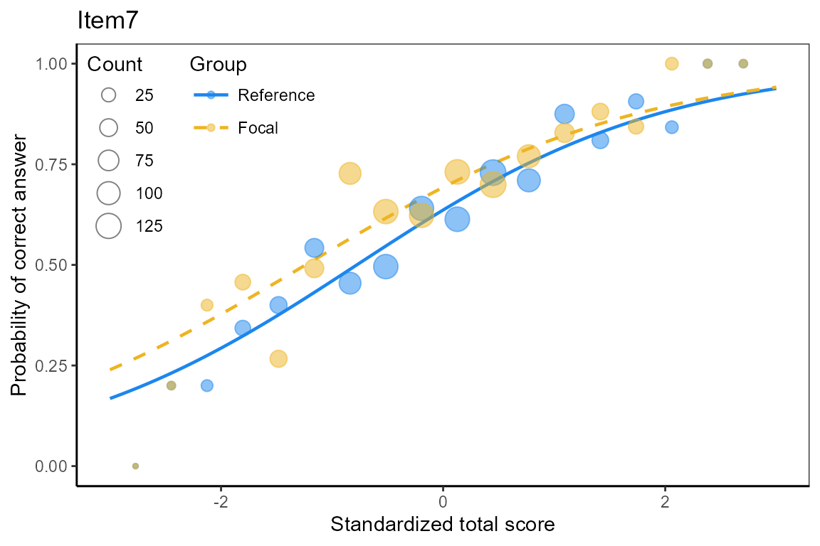

## 
## $Item19